Street Slopes Of Los Angeles

Project Background

For the LADOT Play Streets Program, I was asked if we had a layer that had the following information:

Street Classification
Street Width
Street Slope

The street classification system is part of the street centerline file, maintained by the Los Angeles Department of Public Works Bureau of Engineering and available at the City’s GeoHub here. Street width is contained in a slightly different version of the same centerline file, maintained by the Bureau of Street Services, and available as part of the ‘Street Pavement Condition’ layer on the City’s GeoHub here.

However, there is not readily available layer with street slope already calculated, so I decided to create one myself, using this blog post as a guide. The author, Stephen Von Worley, combined the National Elevation Dataset’s 1/3-second data with the OpenStreetMap grid to produce his result. For this project, I combined the same elevation data with the two layers I mentioned above. Another option in R that I could have pursued included the R package elevatr, which includes queries for elevation data for a bunch of different APIs. Most of the APIs don’t provide access to Digital Elevation Models, which is the most precise elevation data, and definitely necessary for this project. Mapzen, though it does provide API access to raster layers and DEM-based querying API, it has rate limits, so in this case it was just easier to download the DEM raste data and query from there.

Before starting this project, I went ahead and downloaded the two street centerline shapefiles as well as the “USGS NED 1/3 arc-second 2013 1 x 1 degree ArcGrid” elevation data. For the City of Los Angeles, I needed to download two data elevation tiles: n35w119 (Northern LA), and n34w119 (Southern LA). These NED data are at resolutions of 1/3 arc-second (approx. 10 meters) and in some areas at 1/9 arc-second (approx. 3 feet). This is precise enough for the task at hand.

Project Plan

In order to calculate the slope for each street segment, my plan was to calculate the elevation at each end point of the street segment. I could generate an endpoint file from the centerline network, but there is already one available on the GeoHub here. This intersections layer has IDs that can be easily joined to the street centerline file for the slope calculation.

I originally wanted to use the BSS PCI layer features and join the relevant attributes of the BOE centerline layer to the BSS features. After doing the first exercise, however, I realized that the two layers weren’t quite as compatable as I thought. My linking ID, ‘SECT_ID’ is actually a 1:many join with the BOE centerline – there are several cases where there is the same ‘SECT_ID’ for multiple line features. Unfortunately, to my knowledge, there is not an ID that provides a 1:1 join between the BOE and BSS centerline layers. After seeing some confusing results, I decided I needed to pick one to primarily rely on. If I did the BSS, I would need to calculate the endpoints of each segment, and then derive the elevation from there. If I went with BOE, I would need to calculate the length of each segment. I decided to go with BOE as the primary centerline file, and then just pull the BSS file for the street width later.

Project Tools

sf support for simple features; here is a good overview of the package
raster For the analysis of the elevation data
tidyverse Collection of R packages for datascience, including tidyr and dplyr
leaflet for viewing our output on a web map

# load libraries
library(sf, quietly = TRUE, warn.conflicts = FALSE)

## Linking to GEOS 3.6.1, GDAL 2.2.0, proj.4 4.9.3

library(dplyr, quietly = TRUE, warn.conflicts = FALSE)

## Warning: package 'dplyr' was built under R version 3.4.2

library(leaflet, quietly = TRUE, warn.conflicts = FALSE)
library(geosphere, quietly = TRUE, warn.conflicts = FALSE)

## Warning: package 'geosphere' was built under R version 3.4.2

# import street data
bss <- st_read("Data/Street_Pavement_Condition.shp",quiet=TRUE)
boe <- st_read("C:/Users/Tim/Documents/data/street-slope-la/Streets_Centerline/Streets_Centerline.shp", quiet=TRUE)
int <- st_read("Data/Intersections.shp", quiet=TRUE)

Explore the Data

BOE Centerline

glimpse(boe)

## Observations: 84,186
## Variables: 39
## $ OBJECTID   <dbl> 1, 2, 3, 4, 5, 6, 7, 8, 9, 10, 11, 12, 13, 14, 15, ...
## $ ASSETID    <dbl> 168, 169, 170, 171, 172, 173, 174, 175, 176, 177, 1...
## $ INT_ID_FRO <dbl> 4176, 4299, 4373, 4465, 4078, 4149, 4479, 4883, 489...
## $ INT_ID_TO  <dbl> 4259, 1843, 4390, 4488, 4117, 4159, 4624, 4890, 489...
## $ STNUM      <dbl> 1736, 959, 7854, 3463, 2412, 1004, 8609, 6240, 7935...
## $ MAPSHEET   <fctr> 099B209, 088-5A199, 120B177, 117B181, 084B209, 099...
## $ ID         <dbl> 7392, 7417, 7460, 7585, 7015, 7049, 7762, 8129, 813...
## $ ADRF       <dbl> 8301, 701, 2901, 3601, 11501, 1001, 5965, 4601, 440...
## $ ADRT       <dbl> 8399, 799, 2929, 3799, 11599, 1199, 5999, 4699, 479...
## $ ZIP_R      <dbl> 90001, 90044, 90016, 90016, 90059, 90044, 90016, 90...
## $ ADLF       <dbl> 8300, 700, 2900, 3600, 11500, 1000, 5964, 4600, 440...
## $ ADLT       <dbl> 8398, 798, 2928, 3798, 11598, 1198, 5998, 4698, 479...
## $ ZIP_L      <dbl> 90001, 90044, 90016, 90016, 90059, 90044, 90016, 90...
## $ TDIR       <fctr> S, W, S, S, S, W, W, S, S, S, W, S, W, W, S, S, S,...
## $ STNAME     <fctr> WADSWORTH, 110TH, COCHRAN, POTOMAC, SUCCESS, 82ND,...
## $ STSFX      <fctr> AVE, ST, AVE, AVE, AVE, ST, ST, PL, ST, AVE, ST, A...
## $ SFXDIR     <fctr> NA, NA, NA, NA, NA, NA, NA, NA, NA, NA, NA, NA, NA...
## $ STNAME_A   <fctr> NA, NA, NA, NA, NA, NA, NA, NA, NA, NA, NA, NA, NA...
## $ STSFX_A    <fctr> NA, NA, NA, NA, NA, NA, NA, NA, NA, NA, NA, NA, NA...
## $ STATUS     <fctr> O, O, O, O, O, O, O, O, O, O, O, O, O, O, O, O, O,...
## $ TEMP_      <fctr> NA, NA, NA, NA, NA, NA, NA, NA, NA, NA, NA, NA, NA...
## $ SECT_ID    <fctr> 5776100, 6773300, 1229900, 4363900, 5149200, 66710...
## $ DEDRQ      <dbl> 1, 1, 1, 1, 1, 1, 1, 1, 1, 1, 1, 2, 1, 1, 1, 1, 1, ...
## $ REMARKS    <fctr> NA, NA, NA, NA, NA, NA, NA, NA, NA, NA, NA, NA, NA...
## $ SV_STATUS  <fctr> NA, NA, NA, NA, NA, NA, NA, NA, NA, NA, NA, NA, NA...
## $ ST_SUBTYPE <dbl> 1, 1, 1, 1, 1, 1, 1, 1, 1, 1, 1, 1, 1, 1, 1, 1, 1, ...
## $ CRTN_DT    <fctr> 1995-04-06T00:00:00.000Z, 1995-03-24T00:00:00.000Z...
## $ LST_MODF_D <fctr> NA, NA, NA, NA, NA, NA, NA, NA, NA, NA, NA, NA, NA...
## $ OLD_STREET <fctr> Local Street, Local Street, Local Street, Local St...
## $ PLANNING_S <fctr> NA, NA, NA, NA, NA, NA, NA, NA, NA, NA, NA, NA, NA...
## $ DEDRQ_DESC <fctr> No, No, No, No, No, No, No, No, No, No, No, Yes, N...
## $ TOOLTIP    <fctr> WADSWORTH AVE\nStreet Designation: Local Street - ...
## $ NLA_URL    <fctr> navigatela/reports/centerline_mb.cfm?pk=168&t=5776...
## $ Planning_A <dbl> 168, 169, 170, 171, 172, 173, 174, 175, 176, 177, 1...
## $ TYPE       <dbl> 70, 70, 70, 70, 70, 70, 70, 60, 70, 70, 60, 40, 70,...
## $ MODIFIED   <dbl> 0, 0, 0, 0, 0, 0, 0, 0, 0, 0, 0, 0, 0, 1, 0, 0, 0, ...
## $ Street_Des <fctr> Local Street - Standard, Local Street - Standard, ...
## $ Street_D_1 <fctr> Local Street - Standard, Local Street - Standard, ...
## $ geometry   <simple_feature> MULTILINESTRING ((-118.2585..., MULTILIN...

BSS Centerline / Street Pavement Condition

glimpse(bss)

## Observations: 72,113
## Variables: 18
## $ FID        <dbl> 1001, 1002, 1003, 1004, 1005, 1006, 1007, 1008, 100...
## $ SECT_ID    <fctr> 5542400, 5541300, 5541100, 3792300, 4688700, 32909...
## $ STREET_DES <fctr> Secondary Highway, Secondary Highway, Secondary Hi...
## $ PRIME      <fctr> VANOWEN ST, VANOWEN ST, VANOWEN ST, MORSE AVE, ST ...
## $ NAME       <fctr> VANOWEN ST, VANOWEN ST, VANOWEN ST, MORSE AV, SAIN...
## $ OTHER      <fctr> NA, NA, NA, NA, NA, NA, LITTLE, NA, NA, NA, NA, NA...
## $ FROM_      <fctr> WOODMAN AV, GOODLAND AV, BABCOCK AV, VANOWEN ST, V...
## $ TO_        <fctr> MAMMOTH AV, COLDWATER CANYON AV, BELLAIRE AV, WELB...
## $ SURFACE    <fctr> AS, AS, AS, AS, AS, AS, AS, AS, PC, AS, AS, AP, AS...
## $ SURF1      <fctr> Asphalt, Asphalt, Asphalt, Asphalt, Asphalt, Aspha...
## $ STREET_TYP <fctr> SE, SE, SE, LO, LO, LO, SE, LO, LO, LO, LO, SE, LO...
## $ ST_TYPE    <fctr> Select, Select, Select, Local, Local, Local, Selec...
## $ NEWW_CONDI <dbl> 100, 70, 69, 91, 100, 89, 73, 90, 86, 67, 100, 90, ...
## $ STATUS_2   <fctr> Good, Fair, Fair, Good, Good, Good, Good, Good, Go...
## $ ZLENGTH    <dbl> 325, 570, 650, 310, 660, 1955, 1150, 270, 900, 380,...
## $ ZWIDTH     <dbl> 65, 66, 66, 36, 36, 36, 60, 40, 27, 36, 46, 62, 40,...
## $ Shape__Len <dbl> 0.0010913980, 0.0018651708, 0.0021641328, 0.0008528...
## $ geometry   <simple_feature> LINESTRING (-118.4312657132..., LINESTRI...

Data Prep

For the centerline files, both have quite a bit of unneeded information that we can trim out when we do the merge. Since the BSS version of the centerline file contains the street width and the BOE version contains the street classification, we need to merge them (and trim out any other unneeded columns) into one street centerline file. The BSS centerline file is slightly more restrictive – only containing streets that are maintained by the City of Los Angeles – so it will have fewer streets compared to the BOE one. I’ll merge the BOE file with that one.

Note: Once I started bringing in the raster data, I began getting an error while runing the select() function. I found out from this blog post that the error is a result of several packages having a select() function (in this case the function from the raster package is superceding the dplyr one). The solution is simple – make sure to explicitly call out which package you are using with following syntax: package::function()

# trim bss centerline
bss <- bss %>%
  dplyr::select(SECT_ID, PRIME, FROM_, TO_, SURF1, ZLENGTH, ZWIDTH, geometry) %>%
  rename(sect.id = 'SECT_ID',
         street = 'PRIME',
         from = 'FROM_',
         to = 'TO_',
         surface = 'SURF1',
         length.ft = 'ZLENGTH',
         width.ft = 'ZWIDTH',
         geom = 'geometry') %>%
  mutate(sect.id = as.character(sect.id)) %>%
  st_set_geometry(NULL)


# trim boe centerline
boe <- boe %>%
  dplyr::select(ASSETID,
                INT_ID_FRO,
                INT_ID_TO,
                SECT_ID,
                STNAME,
                OLD_STREET,
                Street_Des) %>%
  rename(asset.id = 'ASSETID',
         fromint.id = 'INT_ID_FRO',
         toint.id = 'INT_ID_TO',
         sect.id = 'SECT_ID',
         street = 'STNAME',
         old.desig = 'OLD_STREET',
         new.desig = 'Street_Des') %>%
  mutate(sect.id = as.character(sect.id))

For the intersection layer, the I’m just going to trim away unneeded columns. First, a glimpse:

glimpse(int)

## Observations: 60,627
## Variables: 17
## $ OBJECTID   <dbl> 1001, 1002, 1003, 1004, 1005, 1006, 1007, 1008, 100...
## $ ASSETID    <dbl> 96967, 96968, 96969, 96970, 96971, 96972, 96973, 96...
## $ CL_NODE_ID <dbl> 13589, 13634, 13660, 15007, 15024, 15030, 15031, 15...
## $ X          <dbl> 6392995, 6406002, 6398905, 6480819, 6479671, 647626...
## $ Y          <dbl> 1839536, 1841805, 1841108, 1861803, 1861156, 186087...
## $ LAT        <dbl> 34.04585, 34.05228, 34.05026, 34.10803, 34.10624, 3...
## $ LON        <dbl> -118.5568, -118.5139, -118.5373, -118.2671, -118.27...
## $ TYPE       <fctr> NA, NA, NA, NA, NA, NA, NA, NA, NA, NA, NA, NA, NA...
## $ CRTN_DT    <fctr> NA, NA, NA, NA, NA, NA, NA, NA, NA, NA, NA, NA, NA...
## $ LST_MODF_D <fctr> NA, NA, NA, NA, NA, NA, NA, NA, NA, NA, NA, NA, NA...
## $ USER_ID    <fctr> NA, NA, NA, NA, NA, NA, NA, NA, NA, NA, NA, NA, NA...
## $ FROM_ST    <fctr> PASEO MIRAMAR, VILLA WOODS PL, ALCIMA AVE, WEST SI...
## $ TO_ST      <fctr> ESPERA AVE, D/E, LAS LOMAS AVE, ROWENA AVE, PANORA...
## $ TOOLTIP    <fctr> PASEO MIRAMAR at ESPERA AVE, VILLA WOODS PL at D/E...
## $ ZIP_CODE   <dbl> 90272, 90272, 90272, 90039, 90039, 90027, 90027, 90...
## $ NLA_URL    <fctr> navigatela/reports/intersection_report.cfm?pk=1358...
## $ geometry   <simple_feature> POINT (-118.556805744008 34..., POINT (-...

Now I’ll trim away the unneeded columns:

int <- int %>%
  dplyr::select(ASSETID, CL_NODE_ID, FROM_ST, TO_ST, X, Y, LAT, LON) %>%
  rename(asset.id = 'ASSETID',
         clnode.id = 'CL_NODE_ID',
         from = 'FROM_ST',
         to = 'TO_ST',
         lat = 'LAT',
         lon = 'LON')

Load Raster Layers

In order to calculate the slope of each street segment, I first need to calculate the elevation at each of these street segment endpoints. In order to get the elevation at each of the endpoints (intersections), I am going to extract this elevation data from the raster elevation image that I pulled from the National Elevation Dataset.

library(raster, quietly = TRUE, warn.conflicts = FALSE)

## Warning: package 'raster' was built under R version 3.4.2

# import elevation data & merge into one raster layer
la_n <- raster("C:/Users/Tim/Documents/data/street-slope-la/n35w119/grdn35w119_13")
la_s <- raster("C:/Users/Tim/Documents/data/street-slope-la/n34w119/grdn34w119_13")
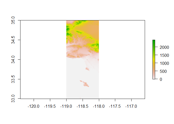
la_elev <- merge(la_n, la_s)

# preview the merged raster
plot(la_elev)

Extract Elevation Data

Note: the sf package was released on CRAN on January 2017, while the latest release of the raster package was back in June 2016. Since there is no interoperability between these two packages, I add the extra step of first converting the sf object into an sp object before working with the raster image. According to the documentation, the elevation values are in meters.

# cast as sp object, extract elevation, convert back to sf object
int_sp <- as(int, "Spatial")
int_elev <- extract(la_elev,
                    int_sp,
                    method='simple')

## Warning in .local(x, y, ...): Transforming SpatialPoints to the CRS of the
## Raster

int_elev <- cbind(int, int_elev)
int_elev <- int_elev %>%
  dplyr::select(clnode.id,
                lat,
                lon,
                int_elev) %>%
  st_set_geometry(NULL)

glimpse(int_elev)

## Observations: 60,627
## Variables: 4
## $ clnode.id <dbl> 13589, 13634, 13660, 15007, 15024, 15030, 15031, 150...
## $ lat       <dbl> 34.04585, 34.05228, 34.05026, 34.10803, 34.10624, 34...
## $ lon       <dbl> -118.5568, -118.5139, -118.5373, -118.2671, -118.270...
## $ int_elev  <dbl> 113.78664, 118.57660, 111.74510, 137.62737, 138.3995...

Street Slope

Now that I have the elevation at each of the intersection points, I can calculate the slope of the each street segment by joining the intersection to the (updated) street centerline file. I need to do the join twice – once for each side of the street. Before that though, I am going to calcualte the length of the BOE segment, which also requires projecting it. During this process, I am also going to filter out any of the private / closed / unknown roads.

streets <- boe %>% 
  mutate(len = st_length(boe)) %>% # get length
  inner_join(int_elev, by=c("fromint.id" = "clnode.id")) %>%
  rename(from.elev = "int_elev") %>%
  inner_join(int_elev, by=c("toint.id" = "clnode.id")) %>%
  rename(to.elev = "int_elev",
         from.lat = "lat.x",
         from.lon = "lon.x",
         to.lat = "lat.y",
         to.lon = "lon.y") %>%
  mutate(slope = (abs((from.elev - to.elev))/(as.numeric(len)))*100) %>% # Slope
  filter(!sect.id %in% c('closed', 'private', 'none', NA, 'outside')) %>%
  filter(!old.desig %in% c('Unknown Type or Closed Street',NA)) %>%
  filter(as.numeric(len) > 50)

At this point I’m also going to attach the street widths from the BSS file. Joining by Section ID (because it is a 1:many join) will result in duplicate rows if there are multiple matches. I could do a semi_join, but this really only filters out the rows of x, without bringing over the columns in y. Instead, I’ll do a left-join and then follow it with a filter for unique values (over the AssetID column).

# semi join boe <- bss
streets <- streets %>%
  left_join(bss, by='sect.id') %>% # join to bss
  dplyr::select(-street.y, -from, -to, -surface, -length.ft) %>% # only keep width
  rename(street = 'street.x') %>%
  distinct(asset.id, .keep_all=TRUE) #unique assetIDs, but keep all cols

Steepest streets in LA?

Let’s take a look at the streets in LA with the highest grade. For this exercise, I wanted to look at segments that were at least 150m long.

# Sort by slope
streets %>%
  mutate(From = paste0("(", from.lat, ",", from.lon,")"),
         To = paste0("(", to.lat, ",", to.lon, ")")) %>%
  dplyr::select(street, slope, len, From, To) %>%
  rename(Length = 'len',
         Slope = 'slope') %>%
  filter(as.numeric(Length) > 150) %>%
  arrange(desc(Slope)) %>%
  head() %>%
  st_set_geometry(NULL) 

##                  street    Slope     Length                        From
## 1                 MACEO 37.78626 202.2191 m (34.09538018,-118.22111464)
## 2               ESCALON 33.93751 158.3219 m (34.13207889,-118.50359726)
## 3                 QUITO 30.83224 270.1126 m (34.10605929,-118.44709108)
## 4                OLETHA 30.51338 211.0095 m  (34.1075104,-118.44697152)
## 5 AVENIDA DE SANTA YNEZ 29.57405 163.2636 m (34.07081161,-118.55832252)
## 6               STOWELL 27.80471 198.5857 m (34.11143116,-118.43899103)
##                            To
## 1  (34.09650793,-118.2193929)
## 2   (34.132951,-118.50231599)
## 3 (34.10686739,-118.44977359)
## 4 (34.10756522,-118.44908363)
## 5 (34.06964038,-118.55925175)
## 6 (34.11090389,-118.44005643)

Top 5 Winners listed below:

Mateo: 37.78% This is actually not a true street! It has been permitted for development (which is why the BOE centerline contains the outline for the street), but it doesn’t count for our purposes.

Escalon: 33.93% The winner is out in Encino, just above Mulholland Dr.
Quito: 30.83% This street exists, and is public, but too narrow for Google car to have gone up.
Oletha: 30.51% This is just one street down from Quito in the same Beverly Glen neighborhood.
Avenida De Santa Ynez: 29.57% Also on the westside, out near Malibu.
Stowell: 27.80% Beverly Glen neighorhood.

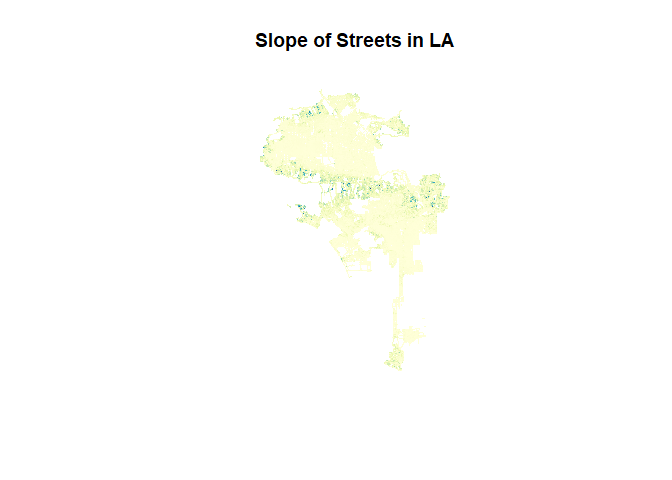
The Map

The map of the final data set! Unsurprisngly, most of the higher sloped streets are around the Hollywood Hills / Porter Ranch / Northeast LA regions.

# Create Color Palette
pal <- colorNumeric(
  palette = "YlGnBu",
  domain = streets$slope
)

# Create the map
plot(x = streets["slope"],
     main = "Slope of Streets in LA",
     col = pal(streets$slope)
     )